Types of Control Systems and Their Industrial Applications

What is a Control System?

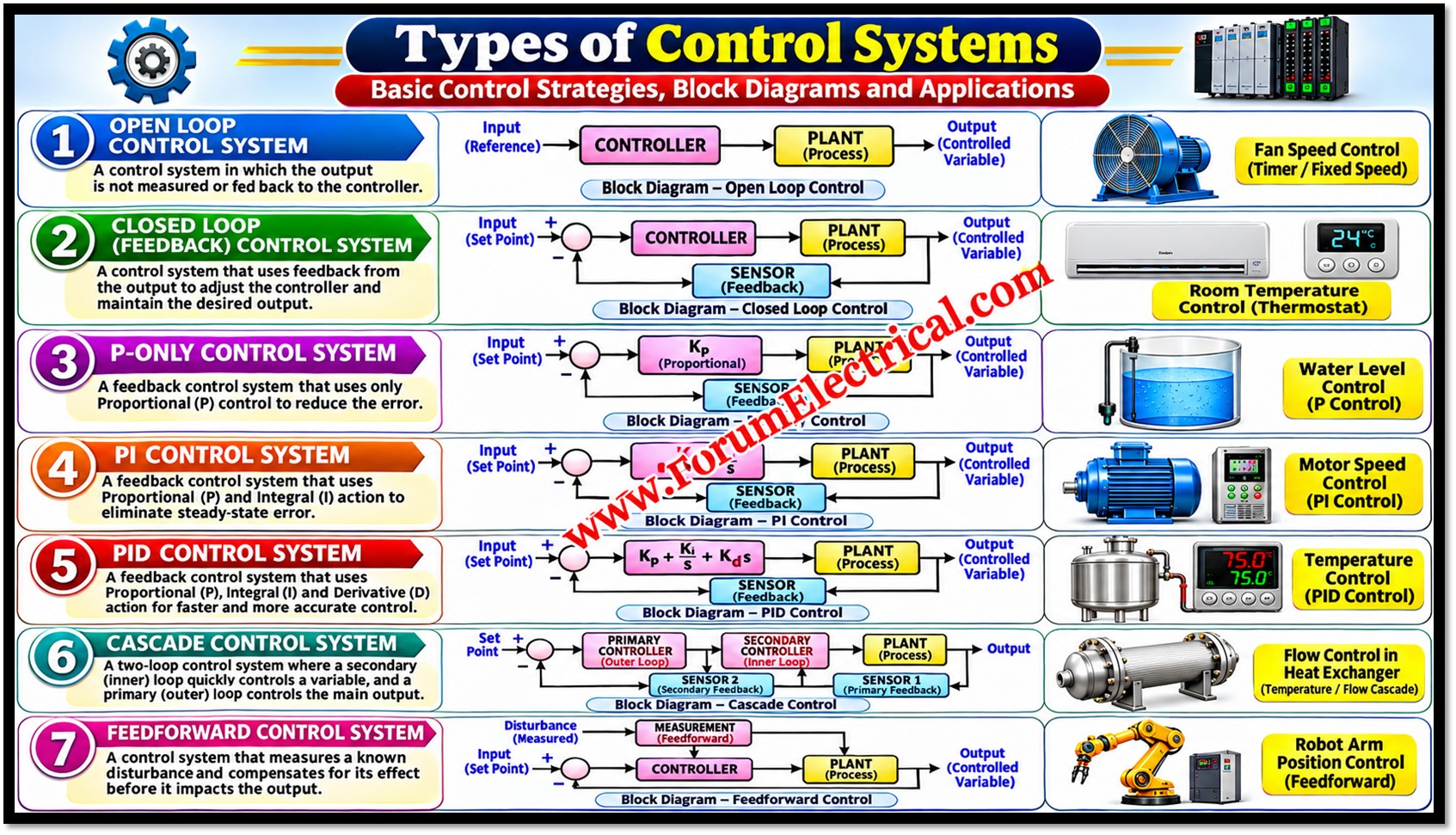
Control systems regulate the operation of machines and industrial processes by manipulating one (or) more process variables so that the process achieves the desired performance, accuracy and stability. 

They are the foundation of modern industrial automation and are implemented in PLCs, DCS, SCADA systems, process instrumentation, robotics & motor drives.

Types of Control Systems

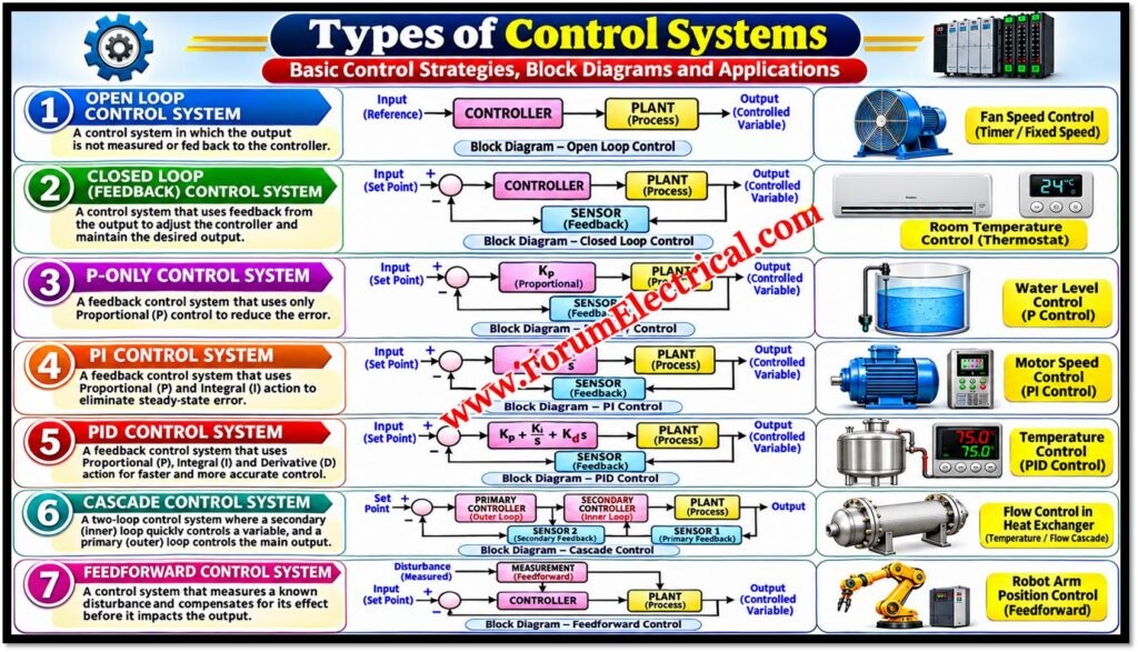
This post analyses 7 fundamental control strategies: 

1. Open-Loop Control System, 
2. Closed-Loop Control System, 
3. Proportional (P) Controller, 
4. Proportional-Integral (PI) Controller, 
5. Proportional-Integral-Derivative (PID) Controller, 
6. Cascade Control System and 
7. Feedforward Control System. 

For each, it explains the operating principle, key characteristics, advantages, limitations and typical industrial use.

Basic Terminology

Term	Meaning
Setpoint (SP, r)	The desired value of the controlled variable.
Process variable (PV, y)	The actual measured value of the controlled variable (the output).
Error (e)	The difference between setpoint and process variable: e(t) = r(t) − y(t).
Controller output (u)	The signal sent by the controller to the final control element.
Manipulated variable	The quantity adjusted to influence the process (e.g., valve position, steam flow, drive frequency).
Disturbance (d)	An unwanted input that pushes the process variable away from the setpoint (e.g., load or supply changes).
Final control element	The device that acts on the process, such as a control valve, damper, heater or variable-frequency drive.
Sensor / transmitter	The device that measures the process variable and sends the signal to the controller.
Steady-state error (offset)	The remaining difference between setpoint and process variable after transients have died out.

Principle of Control Strategies

Strategy	Key Principle	Main limitation	Example
Open-loop	No output feedback; action independent of output	Cannot compensate disturbances	Timer-based washing machine
Closed-loop	Feedback compares output with setpoint	Needs sensors; can become unstable if poorly designed	Automatic room temperature control
P	Output proportional to instantaneous error	May retain steady-state error	Industrial process temperature control
PI	Proportional + integral action	Slower response; integral windup risk	VFD motor speed control
PID	Proportional + integral + derivative	Requires tuning; derivative amplifies noise	Industrial temperature and pressure control
Cascade	Primary loop sets setpoint of secondary loop	Needs an additional measurement and more tuning	Heat exchanger temperature with inner flow loop
Feedforward	Measures disturbance and acts before its effect appears	Needs model and disturbance measurement	Boiler feedwater flow vs. steam demand

1). Open-Loop Control System

Principle

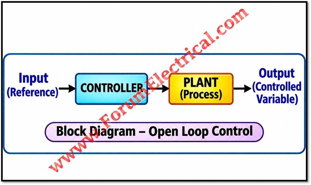
An open loop control system operates without any output feedback.

The control action is determined only by the input (and a predetermined sequence or model) and is independent of the actual output. 

The system does not measure the result of its action and therefore cannot know whether the desired output was achieved.

Input (r)  →  Controller  →  Actuator  →  Process  →  Output (y)     (no return path)

Characteristics

• Control action is independent of the actual output.
• Simple in structure, with few components and low cost.
• Generally stable, because there is no feedback loop that can cause instability.
• Accuracy depends on prior calibration of the system and on the process behaving predictably.
• Cannot automatically compensate for disturbances or changes in process parameters.

Advantages and Limitations

• Advantages: simple, economical, easy to design and maintain, no sensor required.
• Limitations: any disturbance, wear or parameter drift directly causes output error; the error is neither detected nor corrected.

Example

A timer based washing machine runs the wash, rinse and spin stages for fixed durations. 

It does not measure how clean the clothes are and the outcome depends only on the preset timing. 

The same principle applies to simple conveyor timers, fixed-sequence batch operations and traffic lights on fixed timing.

2). Closed-Loop Control System

Principle

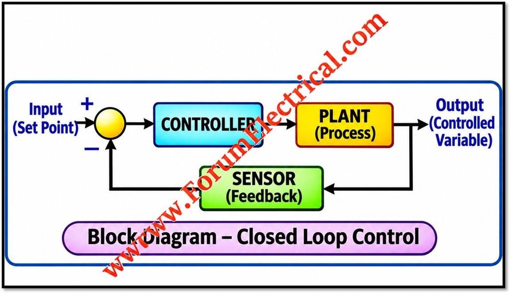
A closed-loop (feedback) control system uses sensors to measure the actual output and compares it with the setpoint. 

The resulting error signal is processed by the controller which automatically adjusts the control action to reduce the error.

e(t) = r(t) − y(t)          

u(t) = f( e(t) )

Setpoint → (+/−) → Controller → Actuator → Process → Output  ↩ Sensor feedback to the comparator

Characteristics

• Continuously compares across the measured output with setpoint.
• Corrects errors automatically, including those caused by unmeasured disturbances.
• Reduces sensitivity to changes in process parameters.
• Requires sensors and a more complex structure than open-loop control.
• Poor design (excessive gain, delays) can cause oscillation or instability, so stability must be considered.

Industrial Example

Automatic room temperature control: a temperature sensor measures the room temperature, the thermostat or controller compares it with the setpoint, and the heating or cooling output is adjusted according to the error. 

This feedback principle is the basis of the P, PI and PID controllers.

Difference between Open-Loop and Closed-Loop Control System

Open-Loop vs. Closed-Loop

Aspect	Open-loop	Closed-loop
Feedback	None	Yes, from sensors
Disturbance compensation	No	Yes, automatic
Accuracy	Depends on calibration	Generally higher
Complexity and cost	Low	Higher
Stability concern	Minimal	Must be designed and tuned for stability
Typical use	Predictable, fixed-sequence tasks	Processes needing accuracy and regulation

3). Proportional (P) Controller

Principle

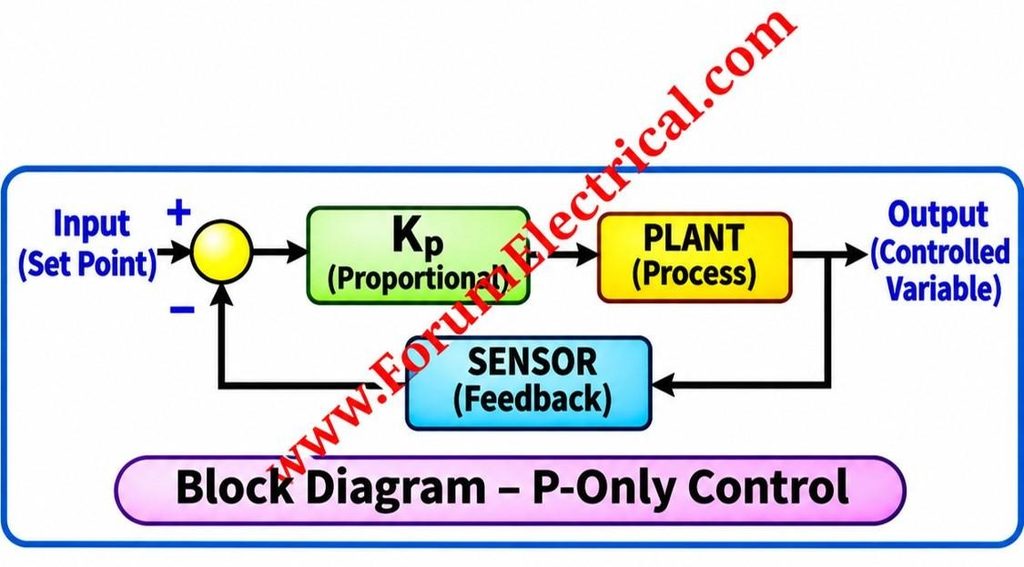
A proportional controller used to generate a control output proportional to the instantaneous (quick) error.

A larger error produces a larger corrective action.

u(t) = Kp · e(t) + u₀

Here 

Kp – Proportional gain and 

u₀ – Bias (output when error is zero). 

In many industrial controllers the gain is also expressed as proportional band: PB (%) = 100 / Kp when the signals are normalised to percent of span.

Characteristics

• Provides a fast response, because the output reacts immediately to the current error.
• May retain a steady-state error (offset). Many processes need a non-zero controller output to hold the setpoint, and a pure P controller produces that output only if a non-zero error exists.
• Increasing Kp reduces the offset and speeds up the response, but excessive gain increases overshoot and oscillation and can lead to instability.
• Simple to implement and tune, with only one tuning parameter.

For a first-order process with steady-state gain K under a step setpoint change, the closed-loop offset is approximately 1 / (1 + Kp·K) of the step size.

The offset decreases as Kp increases but never becomes exactly zero with proportional action alone.

Industrial Example

Industrial process temperature control where moderate accuracy is acceptable and a small offset can be tolerated. 

P control is also used where a deliberate proportional relationship is wanted, for example in some level-control applications where the level is allowed to vary within a band.

4). Proportional-Integral (PI) Controller

Principle

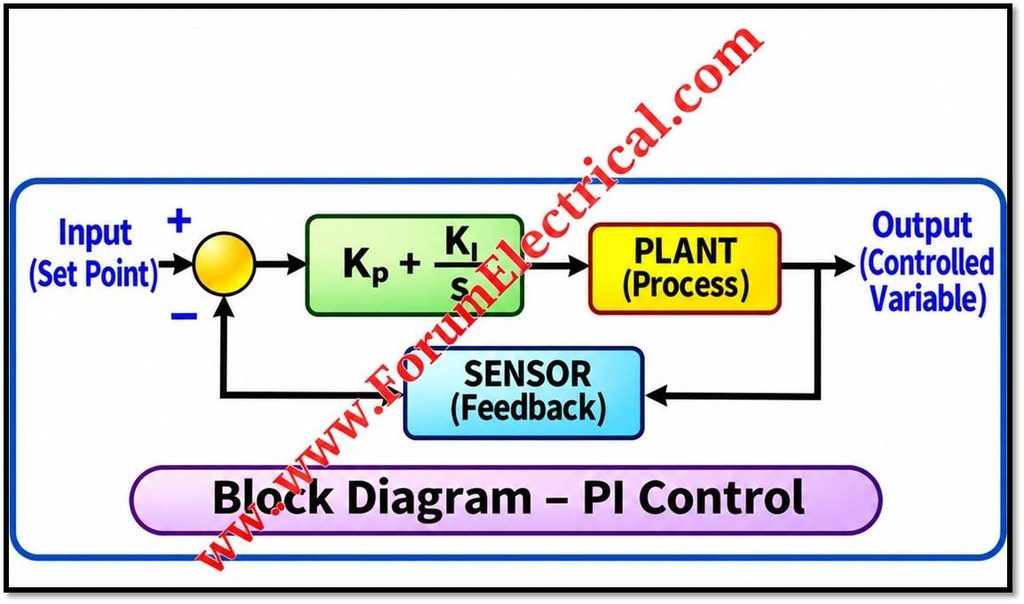
A PI controller combines proportional action with integral action. 

The integral term accumulates the error over time, so a persistent error produces a steadily growing correction until the error is removed.

u(t) = Kp · e(t) + Ki · ∫ e(τ) dτ          

Where Ki = Kp / Ti

Ti is the integral (reset) time. 

A smaller Ti means stronger integral action.

Characteristics

• Reduces or eliminates steady-state error under suitable operating conditions: for a stable loop with a constant setpoint or constant disturbance, the integral action drives the error to zero.
• The proportional term gives immediate response; the integral term removes the remaining offset.
• Integral action adds phase lag, which can reduce stability margins and increase overshoot if it is set too strong.
• Integral windup: if the actuator saturates (e.g., valve fully open or drives at maximum frequency) while the error persists, the integral term keeps growing and causes large overshoot on recovery. Anti-windup measures such as integrator clamping or back-calculation are used to prevent it.
• Because it has no derivative term, it is relatively insensitive to measurement noise, which makes it widely used for noisy or fast loops.

Industrial Example

Variable-frequency drive (VFD) motor speed control: the speed measured by an encoder or tachometer (or estimated by the drive) is compared with the speed reference and a PI controller adjusts the drive output (for example the torque reference in vector control or the frequency command in a closed-loop V/f scheme) to hold the motor speed at the setpoint despite load changes. 

PI control is also used in flow and pressure loops and in pump-speed control.

5). Proportional-Integral-Derivative (PID) Controller

Principle

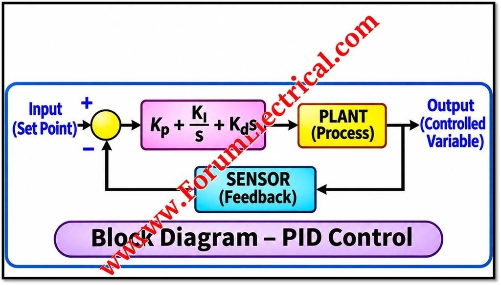
A PID controller combines proportional, integral and derivative actions. 

The derivative term responds to the rate of change of the error providing anticipatory action.

u(t) = Kp · e(t) + Ki · ∫ e(τ) dτ + Kd · de(t)/dt          

Where Ki = Kp/Ti and Kd = Kp·Td

Term	Function	Effect
Proportional (P)	Acts on the present error	Fast response; sets the overall loop gain
Integral (I)	Acts on the accumulated past error	Removes steady-state error
Derivative (D)	Acts on the rate of change (predicted trend) of the error	Adds damping, reduces overshoot, improves dynamic response

Characteristics

• Improves dynamic response and disturbance rejection when properly tuned.
• Requires correct tuning of three parameters (Kp, Ti, Td). Poor tuning can produce sluggish response or oscillation.
• The derivative term amplifies high-frequency measurement noise, so a derivative filter is normally applied. 
• Many implementations apply the derivative action to the measurement rather than the error to avoid “derivative kick” on setpoint changes.
• Anti-windup protection is still needed because of the integral term.
• Derivative action is usually avoided on very noisy signals (such as flow) or on processes dominated by dead time.

Tuning Methods

Common methods include manual trial-and-error, Ziegler–Nichols, Cohen–Coon, lambda (IMC-based) tuning and controller auto-tuning (for example relay-feedback auto-tune). 

The classical Ziegler–Nichols closed-loop (ultimate-gain) rules use the ultimate gain Ku and the oscillation period Pu:

Controller	Kp	Ti	Td
P	0.50 Ku	—	—
PI	0.45 Ku	Pu / 1.2	—
PID	0.60 Ku	Pu / 2	Pu / 8

Ziegler–Nichols settings are a starting point and typically give a fairly aggressive response with noticeable overshoot, so fine-tuning is usually required.

Industrial Example

Industrial temperature and pressure control, for example in furnaces, reactors, boilers, extruders and pressure vessels, where processes have lag and need fast, accurate regulation with good disturbance rejection.

6).Cascade Control System

Principle

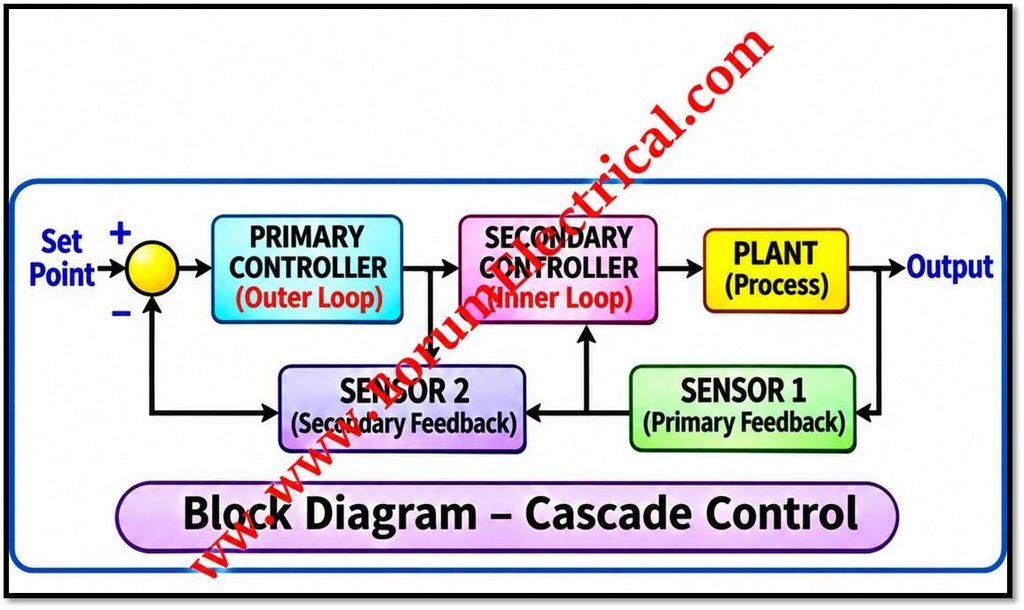
Cascade control uses two feedback loops, a primary (outer or master) loop and a secondary (inner or slave) loop. 

The primary controller measures the main controlled variable and, instead of driving the actuator directly, its output becomes the setpoint of the secondary controller. 

The secondary controller then manipulates the final control element.

SP₁ → Primary controller → (SP₂) → Secondary controller → Final element → Process → PV₁

The secondary loop measures an intermediate variable that responds to the manipulated variable faster than the primary variable does.

Characteristics

• Improves disturbance rejection when the disturbances affect the secondary loop: the inner loop detects and corrects them before they significantly disturb the primary variable.
• The inner loop can also reduce the effect of actuator non-linearity, such as valve characteristic or friction.
• Requires an additional measurement for the secondary variable and an additional controller.
• The secondary loop should be considerably faster than the primary loop (commonly several times faster as a rule of thumb).
• Tuning is performed sequentially: the secondary (inner) loop is tuned first with the primary in manual, and then the primary loop is tuned with the secondary in cascade mode.
• It gives little benefit for disturbances that act only on the primary loop and not on the secondary one.

Industrial Example

Heat exchanger temperature control using an inner flow control loop: 

The primary temperature controller measures the outlet temperature of the process fluid and outputs a flow setpoint for the heating medium (e.g., steam or hot oil). 

The secondary flow controller adjusts the control valve to maintain that flow. Supply pressure disturbances which change the flow are corrected by the flow loop before they reach the outlet temperature.

7). Feedforward Control System

Principle

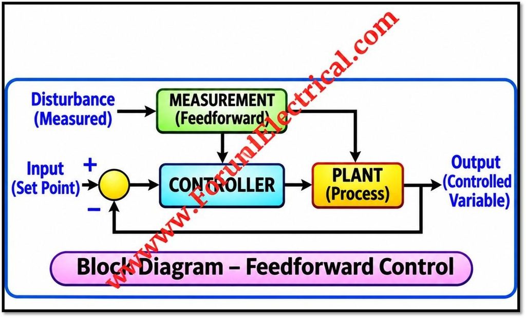
Feedforward control measures a disturbance and applies corrective action before its effects significantly influence the controlled variable. 

Unlike feedback, which acts only after an error has appeared, feedforward acts proactively.

u = u_FB + u_FF          

Ideal feedforward: G_FF(s) = − G_d(s) / G_p(s)

Here G_d(s) is the disturbance-to-output transfer function and G_p(s) is the manipulated-variable-to-output transfer function of the process.

Characteristics

• Requires a suitable process model and a measurement of the disturbance.
• Can greatly reduce the effect of the measured disturbance, since correction is applied before an error develops.
• Cannot correct for unmeasured disturbances or for errors caused by model inaccuracy.
• It is therefore commonly combined with feedback (PID) control, which trims the residual error.
• Dynamic compensation, such as lead-lag and dead-time elements, is often added so the correction arrives at the right time relative to the disturbance.

Industrial Example

Boiler feedwater flow compensation for steam demand changes: steam flow is measured and used to adjust the feedwater flow in advance, so that drum level is maintained when the load changes. 

This is the basis of three-element drum level control, in which steam flow (feedforward), feedwater flow and drum level (feedback) are combined.

Comparative Analysis

Strategy	Feedback	Removes offset	Handles disturbances	Complexity	Typical use
Open-loop	No	No	No	Very low	Fixed sequences
Closed-loop	Yes	Depends on controller	Yes (unmeasured too)	Moderate	General regulation
P	Yes	No (offset remains)	Partly	Low	Simple loops
PI	Yes	Yes	Good	Low–moderate	Speed, flow, pressure
PID	Yes	Yes	Very good if tuned	Moderate	Temperature, pressure
Cascade	Yes (two loops)	Yes (with PI/PID)	Excellent for inner-loop disturbances	Higher	Heat exchangers, reactors
Feedforward	No (usually combined with feedback)	No (needs feedback trim)	Excellent for measured disturbances	Higher	Boilers, load changes

Selection Guidelines

• Use open-loop control when the process is predictable, disturbances are negligible and accuracy requirements are low.
• Use feedback control whenever the output must be regulated accurately despite disturbances.
• Use P control when a small offset is acceptable; use PI when offset must be eliminated; use PID when the process has significant lag and improved dynamic response is needed and noise is manageable.
• Add cascade control when a measurable intermediate variable is affected by major disturbances and responds faster than the primary variable.
• Add feedforward control when a major disturbance can be measured and its effect on the process is reasonably well understood, and keep feedback to remove the remaining error.

Implementation in Industrial Automation

These strategies are widely applied in the following platforms and fields:

• PLCs: PID function blocks for temperature, level, flow and pressure loops, and sequence logic (open-loop style) for machines.
• DCS: Multi-loop process control including cascade and feedforward in refineries, power plants and chemical plants.
• SCADA: Supervisory monitoring, setpoint changes and trending; the control loops typically run in the PLCs or controllers beneath it.
• Process instrumentation: Sensors, transmitters, control valves and positioners that form the measurement and actuation parts of the loops.
• Robotics: Feedback position and velocity loops (commonly PID-based) in joint control.
• Motor drives: PI speed & current loops in VFDs & servo drives.
• Industrial automation in general: Combining the above for accurate, stable and efficient plant operation.

Conclusion

Control strategies range from simple open-loop sequences to feedback controllers (P, PI, PID) and to advanced structures such as cascade and feedforward control. 

Feedback control provides accuracy and automatic correction of errors; integral action removes offset; derivative action improves dynamic response; cascade control improves rejection of inner-loop disturbances; and feedforward control compensates for measured disturbances before they affect the process. 

In practice, these methods are often combined, for instance feedforward with PID trim or cascade PID loops, to achieve the required performance, accuracy and stability in industrial processes.