What is Nyquist Plot?

The Nyquist plot is a continuation of the polar plot, and it is used to determine whether or not a closed-loop control system is stable by varying the value ω from−∞ to ∞.  

In describing the whole frequency response of the open loop transfer function, Nyquist plots are used.

What is Nyquist Plot?

A Nyquist plot (or) Nyquist Diagram is a frequency response diagram used in signal processing and control engineering. Nyquist plots are widely used to evaluate the stability of feedback-controlled control system.

In Cartesian coordinates, the real component of the transfer function is represented on the X-axis, while the imaginary part is plotted on the Y-axis.

The frequency is spanned as a parameter, culminating in a frequency-based graphic.

The same Nyquist plot may be given in polar coordinates, where the transfer function’s gain is the radial coordinate and the phase is the corresponding angular value.

The stability of a feedback control system is determined by locating the roots of the characteristic polynomial (equation) on the s-plane.

If the roots are on the left side of the s-plane, the system is stable. Frequency response approaches, such as the

• Nyquist plot,
• Nichol’s plot, and
• Bode plot,

may be used to assess a system’s relative stability.

The Nyquist stability criteria is used to determine the existence of roots of a certain equation in the s-plane.

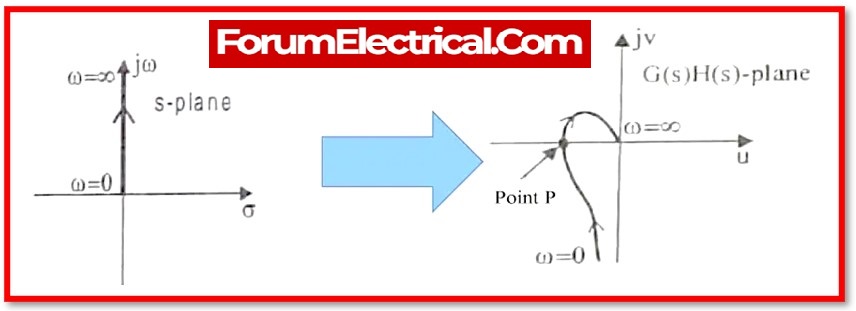
To comprehend a Nyquist plot, must first learn basic terminology. It is worth noting that a contour is a closed route in a complicated plane.

Nyquist Contour or Nyquist Path

The Nyquist contour is an s-plane closed contour that entirely encloses the right-hand half of the s-plane.

To enclose the whole RHS of the s-plane, a large semi-circle route with a diameter along the jω axis and a centre at the origin is formed.

Nyquist Encirclement

Nyquist Encirclement is applied to the radius of the semicircle. If a point is found within a contour, it is said to be encircled by the contour.

Nyquist Mapping

The act of transforming a point in the s-plane into a point in the F(s) plane is known as mapping, and F(s) is known as the mapping function.

Nyquist Stability Criterion

The Nyquist stability criteria is based on the argument principle. It asserts that if the’s’ plane closed route contains P poles & Z zeros, then the associated G(s)H(s) plane must en-circle the origin PZ. times. 

As a result, can express the number of the encirclements N as,

N=P−Z

If the enclosed’s’ plane closed route comprises only poles, the encirclement in the G(s)H(s) plane will be in the opposite direction as the enclosed’s’ plane closed path.

If the contained closed route in the’s’ plane includes exclusively zeros, the encirclement in the G(s)H(s) plane will be in the same direction as the enclosed closed path in the’s’ plane.

Let us now apply the reasoning principle to the full right side of the’s’ plane by making it a closed route. The chosen route is known as the Nyquist contour.

If all of the poles of the transfer function with a closed loop are in the left side of the’s’ plane, the closed loop control system is stable.

As a result, the poles of the close-loop transfer function are the roots of the characteristic equation. The roots get more difficult to obtain as the order (grade) of the characteristic equation grows (increases).

Hence, let us correlate these distinctive equation roots as follows.

The characteristic equation’s poles are the same as the open loop transfer function’s poles.

The characteristic equation zeros are the same as the closed loop transfer function poles.

If there is no open loop pole in the right half of the’s’ plane, we know the open loop control system is stable.

i.e.,P=0⇒N=−Z

If there is no closed loop pole in the right half of the’s’ plane, the closed loop control system is stable.

i.e.,Z=0⇒N=P

Nyquist stability criteria stipulates the number of encirclements around the critical point (1+j0) must be equivalent to the poles of characteristic equation, which are merely the poles of the open-loop transfer function located in the right half of the ‘s’ plane.

The typical equation plane is obtained by shifting the origin to (1+j0).

Nyquist Plot Drawing Instructions

To plot the Nyquist plots, follow the instructions below.

In the’s’ plane, find the poles and zeros of the open loop transfer function G(s)H(s).

Make a polar plot by changing from 0 to infinity. If a pole or zero exists at s = 0, then make a polar plot by changing ω from 0+ to infinity.

Develop the mirror image of the preceding polar plot with values ω ranging from to zero (0 if there is any pole or zero at s=0).

The number of half circles with infinite radius equals the number of poles (or) zeros at the origin. The infinite radius half circle will begin where the polar plot’s mirror image stops.

And this infinite radius half circle will finish where the polar plot begins.

Use the Nyquist stability criteria to determine the stability of the closed-loop control system after producing the Nyquist plot.

If the critical point (-1+j0) is located outside the encirclement, the closed loop control system is completely stable.

Nyquist Plots for Stability Analysis

Based on the values of these parameters, can determine if the control system is stable, moderately stable, or unstable using the Nyquist plots.

• Gain cross-over frequency and phase cross-over frequency
• Phase margin and gain margin

Phase Cross Over Frequency

The phase cross over frequency is the frequency at which the Nyquist plot meets the negative real axis (phase angle is 180⁰). It is represented by the symbol ω_pc.

Gain Cross Over Frequency

The gain cross over frequency is the frequency at which the Nyquist plot has a magnitude of one. It is represented by the symbol  ω_gc.

The stability of the control system is stated below based on the relationship between phase cross over frequency and gain cross over frequency.

The control system is stable if the phase cross over frequency ω_pc is more than the gain cross over frequency ω_gc.

The control system is moderately stable if the phase cross over frequency ω_pc equals the gain cross over frequency ω_gc.

The control system is unstable if the phase cross over frequency ω_pc is lesser than the gain cross over frequency ω_gc.

Gain Margin (GM)

The gain margin GM is equal to the reciprocal of the magnitude (magnitude value) of the Nyquist plot at the phase cross over frequency.

GM=1/M_pc

Where,

M_pc– Magnitude (magnitude value) in normal scale at the phase cross over frequency.

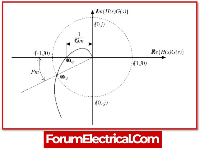
Phase Margin (PM)

PM – Phase Margin is equal to the sum of 1800 & the phase angle at the gain cross-over frequency.

PM=1800+ϕ_gc

Where,

ϕ_gc – Phase angle at the gain cross-over frequency

The stability of the control system is given below based on the relationship between the gain margin & the phase margin.

The control system is stable if the gain margin GM is higher than one & the phase margin PM is positive.

The control system is marginally stable if the gain margin GM equals one and the phase margin PM equals zero degrees.

The control system is unstable if the gain margin GM is less than one and/or the phase margin PM is negative.

Advantages of the Nyquist plot

• It is able to ascertain whether or not the control system is stable.
• In terms of time delay, it performs much better than the root locus. It denotes that the Nyquist plot is capable of effectively working with the time delay that is present in the system.
• It offers a method for making use of the bode plots.
• The frequency response of the open loop transfer function may be determined by it.
• It has the capability of determining the total number of poles that are located on the right side of the s-plane.
• It is also able to determine the system’s degree of relative stability.

Disadvantages of the Nyquist plot

• It employs some sophisticated (complex) mathematical techniques.
• It cannot assess the system’s absolute stability.
• It does not provide an exact count of the number of poles on the right side of the s-plane.

Frequently asked questions:

1). Is Nyquist plot clockwise (or) anticlockwise?

The Nyquist Contour, also known as cN, is a contour that encloses the right half-place and includes the imaginary axis at its centre.

The direction of the Nyquist contour is anticlockwise.

2). Why is Nyquist frequency important?

A discrete signal processing system employs a sampling frequency known as the Nyquist frequency.

This Nyquist frequency is a sort (type) of sampling frequency that is defined as “half of the rate” of the system.

It is the highest frequency (signal) that can be coded for a certain sample rate in order for the signal to be reconstructed. This is the highest frequency that can be coded.

3). What is  Nyquist rate?

In order to prevent the loss of information that is included in the signal, it is necessary to sample at a faster rate if the signal includes high frequency components.

In general, it is important to sample at a frequency that is twice as high as the highest frequency of the signal in order to ensure that all of the information contained in the signal is preserved. This is referred to as the Nyquist rate.

4). What is Nyquist plot in vibration analysis?

A Nyquist plot is a polar plot of a linear system’s frequency response function. It is used to forecast a control system’s stability and performance.

It is also utilised in vibration analysis to derive modal characteristics. The Nyquist plot compares the function’s imaginary versus real components.

5). What is the primary difference between the Nyquist frequency and the sampling frequency?

The Nyquist frequency of a sampled signal is equal to half of the signal’s sampling frequency, and it is the frequency that determines the signal’s bandwidth.

6). What is the main difference between Bode and Nyquist plot?

Bode plots represents a system’s frequency response.

There are two Bode plots:

• one for magnitude (or gain) and
• one for phase.  

The Nyquist plot combines gain & phase into a single complicated plane (one plot) diagram.

7). What is Nyquist plot in the control system?

Nyquist plots are an extension (continuation) of polar plots for determining the stability of closed loop control systems by ranging ω from  −∞ to ∞. .

Nyquist plots are used to show the open loop transfer function’s complete frequency response.

8). What is the Nyquist frequency formula?

The Nyquist frequency is

f_n = 1/2Δt

When presenting spectra for the digital data, the highest frequency visible (shown) is the Nyquist frequency.

9). What is Nyquist’s theorem?

According to Nyquist’s theorem, a periodic signal must be sampled at more than twice the highest frequency component of the signal.

10). What is Nyquist Stability Criterion?

Nyquist stability criterion implies that the number of unstable closed-loop poles equals the number of unstable open-loop poles plus the number of encirclements of the complex function’s origin on the Nyquist plot.